Quickstart
We will be working on a mutagenicity dataset, released by Kazius et
al.. 4337 compounds,
provided as the file mols.sdf, were subjected to the AMES
test. The results are given
in labels.csv. We will clean the molecules, perform a brief chemical
space analysis before finally assessing potential predictive models
built on the data.
Imports
scikit-chem imports all subpackages with the main package, so all we
need to do is import the main package, skchem. We will also need
pandas.
In [3]:
import skchem
import pandas as pd
Loading the data
We can use skchem.read_sdf to import the sdf file:
In [15]:
ms_raw = skchem.read_sdf('mols.sdf'); ms_raw
Out[15]:
name
1728-95-6     <Mol: COc1ccc(-c2nc(-c3ccccc3)c(-c3ccccc3)[nH]...
91-08-7                            <Mol: Cc1c(N=C=O)cccc1N=C=O>
89786-04-9      <Mol: CC1(Cn2ccnn2)C(C(=O)O)N2C(=O)CC2S1(=O)=O>
2439-35-2                               <Mol: C=CC(=O)OCCN(C)C>
95-94-3                             <Mol: Clc1cc(Cl)c(Cl)cc1Cl>
                                    ...
89930-60-9    <Mol: CCCn1cc2c3c(cccc31)C1C=C(C)CN(C)C1C2.O=C...
9002-92-0             <Mol: CCCCCCCCCCCCOCCOCCOCCOCCOCCOCCOCCO>
90597-22-1               <Mol: Nc1ccn(C2C=C(CO)C(O)C2O)c(=O)n1>
924-43-6                                      <Mol: CCC(C)ON=O>
97534-21-9              <Mol: O=C1NC(=S)NC(=O)C1C(=O)Nc1ccccc1>
Name: structure, dtype: object
And pandas to import the labels.
In [5]:
y = pd.read_csv('labels.csv').set_index('name').squeeze(); y
Out[5]:
name
1728-95-6        mutagen
91-08-7          mutagen
89786-04-9    nonmutagen
2439-35-2     nonmutagen
95-94-3       nonmutagen
                 ...
89930-60-9       mutagen
9002-92-0     nonmutagen
90597-22-1    nonmutagen
924-43-6         mutagen
97534-21-9    nonmutagen
Name: Ames test categorisation, dtype: object
We will binarize the labels later.
Quickly check the class balance:
In [6]:
y.value_counts().plot.bar()
Out[6]:
<matplotlib.axes._subplots.AxesSubplot at 0x1219036a0>
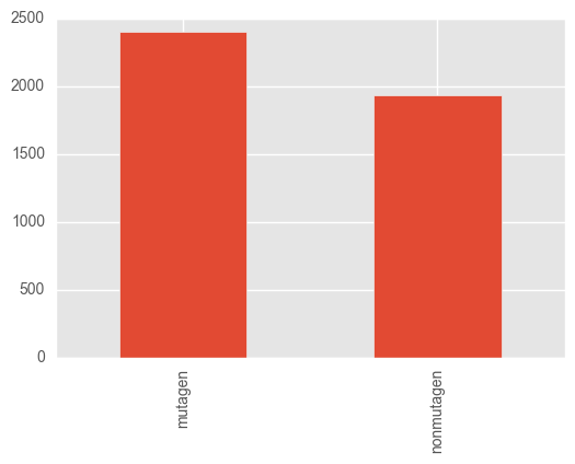
The classes are (mercifully) quite balanced.
Cleaning
The data is unlikely to be canonicalized, and potentially contain broken or difficult molecules, so we will now clean it.
Standardization
The first step is to apply a Transformer to canonicalize the
representations. Specifically, we will use the ChemAxon Standardizer
wrapper. Some compounds are likely to fail this procedure, however they
are likely to still be valid structures, so we will use the
keep_failed configuration option on the object to keep these, rather
than returning a None, or raising an error.
In [6]:
std = skchem.standardizers.ChemAxonStandardizer(keep_failed=True)
In [7]:
ms = std.transform(ms_raw); ms
ChemAxonStandardizer: 100% (4337 of 4337) |#################################################################################################| Elapsed Time: 0:00:22 Time: 0:00:22
Out[7]:
name
1728-95-6     <Mol: COc1ccc(-c2nc(-c3ccccc3)c(-c3ccccc3)[nH]...
91-08-7                            <Mol: Cc1c(N=C=O)cccc1N=C=O>
89786-04-9      <Mol: CC1(Cn2ccnn2)C(C(=O)O)N2C(=O)CC2S1(=O)=O>
2439-35-2                               <Mol: C=CC(=O)OCCN(C)C>
95-94-3                             <Mol: Clc1cc(Cl)c(Cl)cc1Cl>
                                    ...
89930-60-9          <Mol: CCCn1cc2c3c(cccc31)C1C=C(C)CN(C)C1C2>
9002-92-0             <Mol: CCCCCCCCCCCCOCCOCCOCCOCCOCCOCCOCCO>
90597-22-1               <Mol: Nc1ccn(C2C=C(CO)C(O)C2O)c(=O)n1>
924-43-6                                      <Mol: CCC(C)ON=O>
97534-21-9             <Mol: O=C(Nc1ccccc1)c1c(O)nc(=S)[nH]c1O>
Name: structure, dtype: object
Filter undesirable molecules
Next, we will remove molecules that are likely to not work well with the circular descriptors that we will use. These are usually large or inorganic molecules.
To do this, we will use some Filters, which implement the filter
method.
In [8]:
of = skchem.filters.OrganicFilter()

ms, y = of.filter(ms, y)
OrganicFilter: 100% (4337 of 4337) |########################################################################################################| Elapsed Time: 0:00:04 Time: 0:00:04
In [9]:
mf = skchem.filters.MassFilter(above=100, below=900)

ms, y = mf.filter(ms, y)
MassFilter: 100% (4337 of 4337) |###########################################################################################################| Elapsed Time: 0:00:00 Time: 0:00:00
In [10]:
nf = skchem.filters.AtomNumberFilter(above=5, below=100, include_hydrogens=True)

ms, y = nf.filter(ms, y)
AtomNumberFilter: 100% (4068 of 4068) |#####################################################################################################| Elapsed Time: 0:00:00 Time: 0:00:00
Optimize Geometry
We would like to calculate some features that require three dimensional
coordinates, so we will next calculate three dimensional conformers
using the Universal Force Field. Additionally, some compounds may be
unfeasible - these should be dropped from the dataset. In order to do
this, we will use the transform_filter method:
In [11]:
uff = skchem.forcefields.UFF()

ms, y = uff.transform_filter(ms, y)
/Users/rich/projects/scikit-chem/skchem/forcefields/base.py:54: UserWarning: Failed to Embed Molecule 109883-99-0
  warnings.warn(msg)
/Users/rich/projects/scikit-chem/skchem/forcefields/base.py:54: UserWarning: Failed to Embed Molecule 135768-83-1
  warnings.warn(msg)
/Users/rich/projects/scikit-chem/skchem/forcefields/base.py:54: UserWarning: Failed to Embed Molecule 13366-73-9
  warnings.warn(msg)
UFF: 100% (4046 of 4046) |##################################################################################################################| Elapsed Time: 0:01:23 Time: 0:01:23
In [12]:
len(ms)
Out[12]:
4043
As we can see, we get a warning that 3 molecules failed to embed, have
been dropped. If we didn’t care about the warnings, we could have set
the warn_on_fail property to False (or set it using a keyword
argument at initialization). Conversely, if we really cared about
failures, we could have set error_on_fail to True, which would raise
an Error if any Mols failed to embed.
Visualize Chemical Space
scikit-chem adds a custom mol accessor to pandas.Series,
which provides a shorthand for calling methods on all Mols in the
collection. This is analogous to the str accessor:
In [14]:
y.str.get_dummies()
Out[14]:
| mutagen | nonmutagen | |
|---|---|---|
| name | ||
| 1728-95-6 | 1 | 0 |
| 91-08-7 | 1 | 0 |
| 89786-04-9 | 0 | 1 |
| 2439-35-2 | 0 | 1 |
| 95-94-3 | 0 | 1 |
| ... | ... | ... |
| 89930-60-9 | 1 | 0 |
| 9002-92-0 | 0 | 1 |
| 90597-22-1 | 0 | 1 |
| 924-43-6 | 1 | 0 |
| 97534-21-9 | 0 | 1 |
4043 rows × 2 columns
We will use this function to binarize the labels:
In [25]:
y = y.str.get_dummies()['mutagen']
Amongst other options, it is provides access to chemical space plotting functionality. This will featurize the molecules using a passed featurizer (or a string shortcut), and a dimensionality reduction technique to reduce the feature space to two dimensions, which are then plotted. In this example, we use circular Morgan fingerprints, reduced by t-SNE to visualize structural diversity in the dataset.
In [16]:
ms.mol.visualize(fper='morgan',
                 dim_red='tsne', dim_red_kw={'method': 'exact'},
                 c=y,
                 cmap='copper')
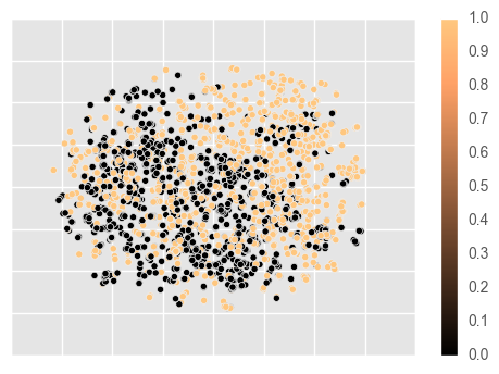
The data appears to be reasonably separable in structural space, so we may suspect that Morgan fingerprints will be a good representation for modelling the data.
Featurizing the data
As previously noted, Morgan fingerprints would be a good fit for this
data. To calculate them, we will use the MorganFeaturizer class,
which is a Transformer.
In [13]:
mf = skchem.descriptors.MorganFeaturizer()

X, y = mf.transform(ms, y); X
MorganFeaturizer: 100% (4043 of 4043) |#####################################################################################################| Elapsed Time: 0:00:00 Time: 0:00:00
Out[13]:
| morgan_fp_idx | 0 | 1 | 2 | 3 | 4 | ... | 2043 | 2044 | 2045 | 2046 | 2047 |
|---|---|---|---|---|---|---|---|---|---|---|---|
| name | |||||||||||
| 1728-95-6 | 0 | 0 | 0 | 0 | 0 | ... | 0 | 0 | 0 | 0 | 0 |
| 91-08-7 | 0 | 0 | 0 | 0 | 0 | ... | 0 | 0 | 0 | 0 | 0 |
| 89786-04-9 | 0 | 0 | 0 | 0 | 0 | ... | 0 | 0 | 0 | 0 | 0 |
| 2439-35-2 | 0 | 0 | 0 | 0 | 0 | ... | 0 | 0 | 0 | 0 | 0 |
| 95-94-3 | 0 | 0 | 0 | 0 | 0 | ... | 0 | 0 | 0 | 0 | 0 |
| ... | ... | ... | ... | ... | ... | ... | ... | ... | ... | ... | ... |
| 89930-60-9 | 0 | 0 | 0 | 0 | 0 | ... | 0 | 0 | 0 | 0 | 0 |
| 9002-92-0 | 0 | 0 | 0 | 0 | 0 | ... | 1 | 0 | 1 | 0 | 0 |
| 90597-22-1 | 0 | 0 | 0 | 0 | 0 | ... | 0 | 0 | 0 | 0 | 0 |
| 924-43-6 | 0 | 0 | 0 | 0 | 0 | ... | 0 | 0 | 0 | 0 | 0 |
| 97534-21-9 | 0 | 0 | 0 | 0 | 0 | ... | 0 | 0 | 0 | 0 | 0 |
4043 rows × 2048 columns
Pipelining
If this process appeared unnecessarily laborious (as it should!),
scikit-chem provides a Pipeline class that will sequentially
apply objects passed to it. For this example, we could have simply
performed:
In [16]:
pipeline = skchem.pipeline.Pipeline([
        skchem.standardizers.ChemAxonStandardizer(keep_failed=True),
        skchem.filters.OrganicFilter(),
        skchem.filters.MassFilter(above=100, below=1000),
        skchem.filters.AtomNumberFilter(above=5, below=100),
        skchem.descriptors.MorganFeaturizer()
])

X, y = pipeline.transform_filter(ms_raw, y)
ChemAxonStandardizer: 100% (4337 of 4337) |#################################################################################################| Elapsed Time: 0:00:23 Time: 0:00:23
OrganicFilter: 100% (4337 of 4337) |########################################################################################################| Elapsed Time: 0:00:04 Time: 0:00:04
MassFilter: 100% (4337 of 4337) |###########################################################################################################| Elapsed Time: 0:00:00 Time: 0:00:00
AtomNumberFilter: 100% (4074 of 4074) |#####################################################################################################| Elapsed Time: 0:00:00 Time: 0:00:00
MorganFeaturizer: 100% (4064 of 4064) |#####################################################################################################| Elapsed Time: 0:00:00 Time: 0:00:00
Modelling the data
In this section, we will try building some basic scikit-learn models on the data.
Partitioning the data
To decide on the best model to use, we should perform some model selection. This will require comparing the relative performance of a selection of candidate molecules each trained on the same train set, and evaluated on a validation set.
In cheminformatics, partitioning datasets usually requires some thought, as chemical datasets usually vastly overrepresent certain scaffolds, and underrepresent others. In order to get as unbiased an estimate of performance as possible, one can either downsample compounds in a region of high density, or artifically favor splits that pool in the same split molecules that are too close in chemical space.
scikit-chem provides this functionality in the SimThresholdSplit
class, which applies single link heirachical clustering to produce a
large number of clusters consisting of highly similar compounds. These
clusters are then randomly assigned to the desired splits, such that no
split contains compounds that are more similar to compounds in any other
split than the clustering threshold.
In [26]:
cv = skchem.cross_validation.SimThresholdSplit(fper=None, n_jobs=4).fit(X)
train, valid, test = cv.split((60, 20, 20))
X_train, X_valid, X_test = X[train], X[valid], X[test]
y_train, y_valid, y_test = y[train], y[valid], y[test]
Model selection
.. todo:: Improve the modelling section: - More features - More models - Grid Searches over skchem cross validation indexes
In [27]:
import sklearn.ensemble
import sklearn.linear_model
import sklearn.naive_bayes
In [28]:
rf = sklearn.ensemble.RandomForestClassifier(n_estimators=100)
nb = sklearn.naive_bayes.BernoulliNB()
lr = sklearn.linear_model.LogisticRegression()
In [30]:
rf_score = rf.fit(X_train, y_train).score(X_valid, y_valid)
nb_score = nb.fit(X_train, y_train).score(X_valid, y_valid)
lr_score = lr.fit(X_train, y_train).score(X_valid, y_valid)

print(rf_score, nb_score, lr_score)
0.850119904077 0.796163069544 0.809352517986
Random Forests appear to work best (although we should have chosen hyperparameters using Random or Grid search). Final value
Assessing the Final performance
In [31]:
rf.fit(X_train.append(X_valid), y_train.append(y_valid)).score(X_test, y_test)
Out[31]:
0.82051282051282048